
Visualizations of Spacetime Curvature
Contents
Overview of the visualization method
Illustration for an oscillating source with symmetry
Illustration for a rotating source
Illustration for a rotating black hole
Overview of the visualization method
The warping of empty spacetime in general relativity is described mathematically in terms of quantities known as curvature tensors. The effects of curvature can be understood most simply by the physical effects it has on nearby observers who synchronize their clocks. As described in more detail in the post here, the tensors at an instant of time can be broken into two matrices throughout space, which measure the tidal stretching and squeezing between two observers for the first matrix and the relative rate of precession of nearby gyroscopes for the second (the so-called electric and magnetic parts, respectively). The stretching and squeezing related to the electric part is the relativistic analog of the tidal gravitational field that produces the ocean tides on the Earth, which are caused by the gravity of the Moon and Sun. The relative precession effect of the magnetic part has no simple analog in non-relativistic physics, but one can understand its effect as a type of gravitationally induced relative twisting of two nearby points, like what happens when one wrings out a wet towel.
Visualizing a matrix is challenging because a matrix contains information about both magnitudes are directions. Because the electric and magnetic curvature tensors have some nice properties (they are symmetric about their diagonal elements), they can always be decomposed into a set of three orthogonal directions and three associated magnitudes (or scales), which sum to zero (these are the so-called eigendirections and the eigenvalues associated with the respective directions). The full information about the curvature can be illustrated by showing the three directions and information about the three scales associated with each of these three directions. The animations and images on this page illustrate a new approach to visualizing these tensors that differs from the original approach described here. This new method is demonstrated below on three spacetimes. Two of them are models of binary black holes radiating gravitational waves far from the black holes and (one simpler two-dimensional example and one fully three-dimensional example), and one is a rotating black hole in isolation.
The visualization technique is as follows. The directions are illustrated by using a set of short orthogonal lines at a number of points distributed uniformly throughout space in the coordinates used (two lines in the 2D case, and three in the 3D case). The length of the line associated with direction with the largest corresponding absolute value of the scale (independent of the sign) is always drawn with the same length. The other line (2D) or lines (3D) corresponding to the other direction(s) is shortened by a factor of the ratio of the absolute values of the smaller scale to the largest scale. Finally, the color of the line (red or blue) tells whether scale associated with that direction is negative or positive. For the electric part, this means that gravity stretches (red) or squeezes (blue) along that direction, and for the magnetic part, it means that gravity causes a relative twisting in the counterclockwise (red) or clockwise (blue) sense about an axis pointing in that direction. The gray-scale, color-density plot gives information about the amplitude of the largest scale (in absolute value) at each point in space. Darker gray colors indicate that the scale is larger in magnitude and lighter gray colors indicate that it is smaller. Return to contents.
Illustration for an oscillating source with symmetry
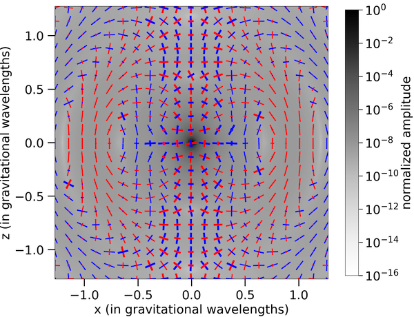
The first example is an oscillating source of gravitational waves that has an axis of symmetry (such a system would arise after the head-on collision of two non-rotating black holes, for example). This case, while not yet observed in our Universe, is a helpful simpler example for demonstrating the visualization technique, because the electric part of the curvature is the same on all the planes that contain the symmetry axis, and two of the three directions always lie within this plane (the third direction is always perpendicular to this plane). Thus, one can visualize essentially all the stretching and squeezing effects throughout space by plotting a single two-dimensional plane. Note, however, that the magnetic part of the curvature does not have this property: it will have directions that point both into and out of this plane. Thus, it will not be illustrated in this first example.
A source like an oscillating, distorted black hole formed from the head-on collision of two non-rotating black holes contains strong stretching and squeezing effects that are related to just the total gravitational mass of the black hole. However, the curvature associated with the total mass of the black hole (the monopole moment) does not produce any gravitational waves; it is only the time-dependent asymmetries that generate gravitational waves (specifically, the quadrupole and higher multipole moments of the system). Even close to the black hole, the effects of the curvature of the total mass often dwarf any effects related to the curvature associated with the gravitational waves. Eventually the curvature related to the waves becomes stronger than that of the total mass, but this typically occurs at very large distances from the source of the waves. Thus, to illustrate the generation of gravitational waves, it is helpful to visualize only the part of the curvature associated with the waves, which is what is done in the two-dimensional visualization here (as well as the three-dimensional one below). Furthermore, only the dominant, quadrupolar part of the waves is illustrated in these cases.
The area visualized contains the region close to the oscillating source out to a distance roughly on the order of a wavelength of the gravitational waves. It thus illustrates how the dynamics of the spacetime curvature close to the source (where the finite light travel time is short, so the source changes almost instantaneously) transitions to the region where the gravitational waves are propagating away from the source and the time delays associated with the light-travel time from the center to that point are significant. This region, sometimes referred to as the induction zone, shows how the time-varying curvature close to the center (or origin) of the plane induces changes in the curvature further away that travel away from the source as gravitational waves. The amplitude of the stretching and squeezing effect falls off rapidly as the distance from the center increases, as is shown in the gray color-scale that rapidly lightens as distance increases from the center of the figure. Return to contents.
Illustration for a rotating source
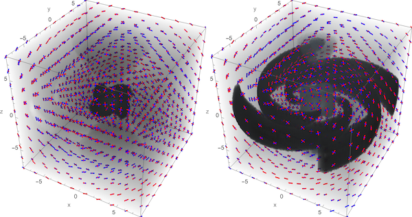
This three-dimensional example again shows the generation of gravitational waves, but this source does not have an axis of rotational symmetry. As a result, there are not generic planes that illustrate the spacetime curvature, and the curvature is best illustrated in all three dimensions. Both the electric and magnetic parts of the curvature will be shown in this visualization. Physically, this example illustrates the part of the spacetime curvature associated with the gravitational waves from two black holes inspiralling on a nearly circular orbit, such as those observed by the LIGO and Virgo detectors. As with the two-dimensional visualization, this three-dimensional visualization shows the curvature generating the waves close to the source. The gravitational waves measured by LIGO and Virgo are frequently a billion billions (1018) gravitational wavelengths away. Thus, the amplitude of the waves is significantly weaker once they reach the Earth.
The image on the left visualizes the electric part of the curvature and the right is the magnetic part. In this case, the scale of the tensor was multiplied by a function of distance from the center so as to remove the decrease in amplitude of the field that occurs far from the source and the rapid growth in amplitude near the origin. This rescaling also helps highlight the angular pattern of the source. Close to the source, the electric part is strongest, and it has a four-lobe pattern typical of a quadrupolar source. In the animation, the pattern rotates rigidly, because near the source the effects of time delays are negligible. In terms of the angular pattern, the field is strongest near the equatorial (x-y) plane and weaker near the poles (along the z axis). At larger distances, however, the effects of the time delays become more important, and the field begins to propagate outward. In terms of the angular pattern, the field becomes stronger near the poles rather than near the equator, which is typical of quadrupolar waves. Finally, in terms of the directions of stretching a squeezing at these larger distances, the radial direction has very little stretching or squeezing, so the two transverse directions are much more prominent. The magnitude of the transverse stretching and squeezing is comparable, which is also typical of that of gravitational waves.
The magnetic part on the right has a somewhat different behavior. The field does not grow quite as strongly as it approaches the origin, so the rigidly rotating part of the field near the center is not the most prominent feature, with the rescaling used in this visualization. The most prominent part, in fact, is in the equatorial plane in the region where the curvature begins to propagate outwards as gravitational waves. This magnetic part of the curvature is induced by the time-varying electric part, analogously to the induction through the displacement current in Maxwell’s equations. Also at larger distances, the field along the polar axis becomes stronger, and it will eventually become the dominant part at even larger distances. The transverse directions are similar to those of the electric part at larger distances, but are rotated by forty-five degrees. This is also typical of gravitational waves. Return to contents.
Illustration for a rotating black hole
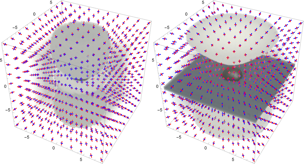
This third example, illustrated above, shows the two types of curvature for a black hole rotating at ninety percent of the maximum value. The electric type (tidal stretching and squeezing) is on the left half of the image and the magnetic type (frame-drag relative twisting) is on the right half of the image. In both images, the event horizon of the black hole is illustrated by a black squashed ellipsoidal surface in the center of each image (it is more obscured by the gray colored region in the left panel than it is in the right panel). The red and blue axes at each point in each image indicate the directions of the stretching and squeezing (left) and twisting (right) effects induced by the curvature of space and time.
The gray-colored volumes in the image on the left illustrate the surfaces of constant largest eigenvalue in magnitude when the radial dependence of the strength of the tidal stretching and squeezing has been scaled out to highlight the angular pattern of the effect. A black hole that is not rotating would have no angular pattern, so the gray regions would be spherical surfaces. Moving far away from the black hole, the surfaces of constant eigenvalue would become these spherical shapes. However, close to the black hole, the effects of stretching and squeezing along the axis of rotation of the black hole differs from that along the plane that passes through the equator of the black hole. This gives rise to the two lobes above and below the black hole (centered around its two poles) and the donut-shaped ring around the equator of the black hole. The lighter gray color here indicates that the tidal effects are larger near the equator than they are close to the poles. The stretching and squeezing is symmetric about the equator of the black hole, so although some of the regions below the equator are obscured from this view point, they are equivalent to those regions that are visualized above the equator.
On the right panel of the image, the frame-drag twisting effects vanish in the equatorial plane passing through the equator of the black hole (shown by the dark plane region) and the twisting effects are largest near the poles, where there are the lighter gray conical-shaped regions. The magnitude of the twisting effect has again been scaled by the distance from the center of the black hole to highlight the angular pattern of the effect. The direction of the rotation is equal and opposite above and below the black hole’s equator. Thus, one does not miss out on any aspect of the visualization by viewing from above, as is done here.1 Return to contents.
-
This material on this page on visualizations is based upon work supported by the National Science Foundation under Grant Number PHY-2011784. Any opinions, findings, and conclusions or recommendations expressed in this material are those of the author and do not necessarily reflect the views of the National Science Foundation. ↩